SOC (soil organic carbon) under regenerative practice approaches a saturation ceiling \(C_{\max}\). The deficit \(D(t) = C_{\max} - C(t)\) closes continuously at rate \(r\):
\(\;D(t) = D_0 \cdot e^{-rt}\), so \(C(t) = C_{\max} - (C_{\max} - C_0)\cdot e^{-rt}\).
Early years (decades 1–2), when \(C(t) \ll C_{\max}\), accumulation looks roughly linear — perfect terrain for the IM lesson's "small \(r\): \(e^{r}\) and \(1+r\) are very close" comparison.
Key numbers students will use
Silvopasture sequestration: Project Drawdown median 9.81 t CO\(_2\)e/ha/yr. Rodale-aligned and meta-analysis estimates: ~2.7–4.8 tC/ha/yr (≈ 9.9–17.6 t CO\(_2\)e/ha/yr depending on tree density).
No-till + cover crops, US Midwest: SOC stock increase 0.36 ± 0.12 Mg/ha/yr (≈ 1.32 t CO\(_2\)e/ha/yr).
4 per 1000 target: 0.4% per year increase in top-30-cm SOC (treaty-style aspirational target).
US cropland total:328 million acres in 2024 (≈ 132.7 million ha). No-till at 38%, cover crops at 4.7% (2022 Ag Census).
Saturation timeline: typical equilibrium reached in 20–50 years; cropland SOC currently averaging only ~30% of saturation capacity.
Rodale 40-yr trial: compost + rotation → up to 2,000 lb C/acre/yr (≈ 2.24 tC/ha/yr) in early decades; conventional tillage loses~300 lb/acre/yr.
Agroforestry footprint: < 2% of US farms; 5,300 acres documented in silvopasture across NJ/PA/NY/New England (145 producers surveyed).
Interventions with measured effect sizes
EQIP (Environmental Quality Incentives Program): $8.45B from IRA over 5 years; cover-crop payment $50–$75/acre; up to 90% cost-share for socially-disadvantaged / beginning farmers. Effect: in 2021, 2.3M acres cover-cropped via EQIP.
CSP (Conservation Stewardship Program): $3.25B from IRA. Largest US conservation program by acres enrolled.
Inflation Reduction Act 2022: $19.5B over 5 yrs to climate-smart ag; +$300M for measurement (Soil Carbon Monitoring Network).
Farmer First Regenerative Pilot (FY2026): States set aside 25% of EQIP/CSP funds for regenerative producers. 5-yr minimum contracts.
Carbon credit markets: Indigo Ag — $60–$100/credit, 75% to farmer; 2M+ verified t CO\(_2\)e since 2022. Nori shut down Sept 2024 (measurement-cost problem).
Silvopasture in Pennsylvania
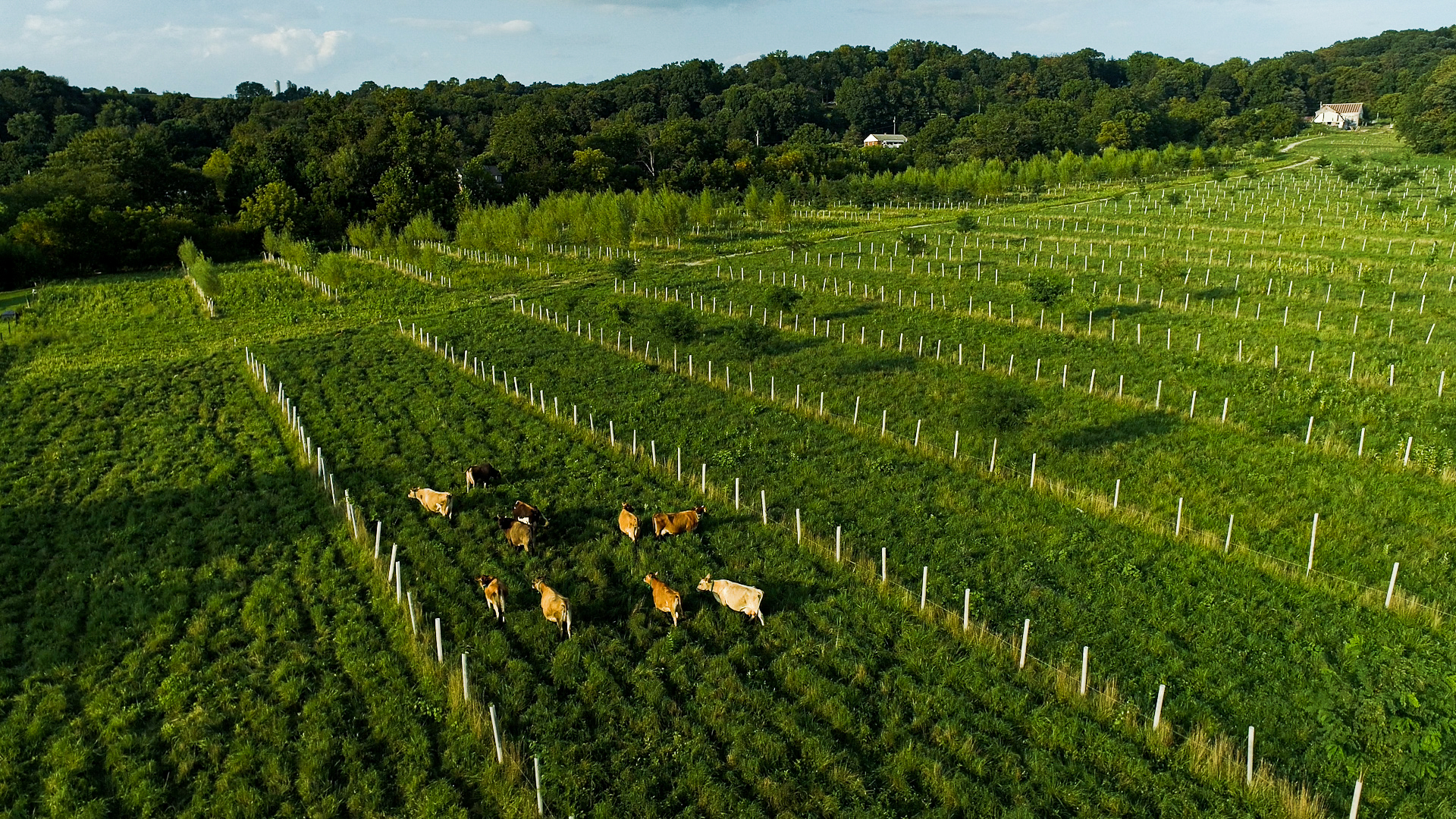
— cattle, grass, and widely-spaced hardwoods on the same acre. Project Drawdown ranks silvopasture among the top 10 climate solutions, sequestering ~9.8 t CO\(_2\)e/ha/yr in living biomass and soil organic carbon. Photo: Savanna Institute, 2023. CC BY-SA 4.0.
What is the difference between "growing 5% per year"
and "growing continuously at 5%" —
and does the distinction
actually change anything?
Standards: HSF-LE.A.4, HSF-LE.B.5, HSA-SSE.A.1.b. The IM lesson introduces base \(e\) and the form \(P_0 \cdot e^{rt}\). Today's wrench: instead of "insect colony" or "1964 US population," the carrier context is soil organic carbon under regenerative agriculture — a model Mr. Bennett's permaculture students will find immediately familiar.
Topic note: Continuous-rate models are how climate scientists actually report sequestration. Not despair-math: cropland SOC currently sits at ~30% of its saturation ceiling, so the deficit is the lever, and the rate \(r\) is set by adoption policy. The agency move at the end is real: federal and state programs measurably move \(r\).
Materials: Scientific or graphing calculators with an \(e^{x}\) key, one per student (warm-up depends on this).
Prep Checklist
☐ Confirm calculators have \(e^{x}\) (usually 2nd → ln).
☐ Open the data packet (top-right) before class to skim numbers.
☐ Activity 3 (graphing) is the IM optional — skip if pacing is tight.
Warm-Up5 min
Do Now — Find \(e\) on your calculator
The number \(e \approx 2.71828\) is a mathematical constant — like \(\pi\). It appears whenever something grows or decays continuously. Find the \(e^{x}\) key on your calculator (usually 2nd → ln).
Complete on your own. Then confirm your answers with a partner.
Evaluate \(e^{0.05}\). You should get approximately 1.0513.
Evaluate \(e^{(0.034)(50)}\). You should get approximately 5.474. (Watch your parentheses.)
Evaluate \(50 \cdot e^{-0.03 \cdot 20}\). You should get approximately 27.44.
5 min total for warm-up + synthesis (slides 2–3). Students do not yet need to interpret these numbers — that is what the rest of the lesson is for. The point of the warm-up is purely technical: get every student's calculator to produce the same value.
Watch for students who type \(e^{0.034 \cdot 50}\) without parentheses and get a wildly wrong answer (the calculator may evaluate \(e^{0.034}\) first, then multiply by 50). Press the parenthesis habit — they will use it for the rest of the unit.
Some calculator models display 2.71828... with different decimal precision; expected answers above use 4-decimal rounding. Do not resolve what \(e\) means here — Activity 1 does that.
Warm-Up · Synthesis2 min
Calculator Check — Quick Discussion
A quick check — if a student got a wildly different answer, the issue is almost always parentheses or the order of operations on the exponent.
“What did you type to get \(e^{(0.034)(50)} \approx 5.474\)?”Type e^( first — then 0.034 × 50 inside — then ). Without the parentheses, many calculators evaluate \(e^{0.034}\) first and multiply by 50, giving ~51.7 instead of 5.474.
“Why does the third one give 27.44 (less than 50)?”The exponent is negative: \(-0.03 \cdot 20 = -0.6\), so \(e^{-0.6} \approx 0.5488\). And \(50 \cdot 0.5488 \approx 27.44\). Negative exponent on \(e\) → the value decays.
click to advance discussion ▶
Two minutes max. Goal: every calculator works. The conceptual move (what does it mean for the rate to be applied "continuously"?) belongs to Activity 1, not here.
Activity 1 · Launch3 min
Same Soil — Two Models
A South Jersey farm transitions a 1-hectare field from conventional corn-soybean to silvopasture — pastured cattle under widely-spaced hardwoods. Year 0: soil organic carbon \(C_0 = 40\) tons/ha. Studies project SOC will grow about 3.4% per year for the first decade or two, until the soil approaches saturation.
Aleena's model
"3.4% applied once at the end of each year."
\(A(t) = 40 \cdot (1.034)^{t}\)
Marcus's model
"3.4% applied continuously, at every moment."
\(M(t) = 40 \cdot e^{0.034\,t}\)
What do you notice? What do you wonder?
Launch (~3 min). Display both models. Ask: "What do you notice? What do you wonder?"
Possible noticings: Same starting value (40). Same rate (3.4%). Different formulas. One has \(1.034\) as the base; the other has \(e\). Marcus's exponent has the rate multiplying the time.
Possible wonderings: Are they the same? Will they predict different SOC values? Why use \(e\)? Which one is "right"?
Do not resolve. Students will fill in a table and graph both functions in work time and discover the difference for themselves. If a student says "they have to be the same — the rate is 3.4% in both," that is exactly the productive struggle the activity is designed to expose.
Activity 1 · Work Time12 min
Problems
Use a calculator to fill in the table for both models. Round to 2 decimals.
What do you notice about \(A(t)\) and \(M(t)\) for small \(t\)? For \(t = 50\)?
Graph both functions on the same axes for \(0 \le t \le 50\). Use a window for \(C\) from 30 to 250.
Marcus says the two graphs look identical. Aleena says they are not. Who is right? Defend your answer.
Try Saying
For small \(t\), the two models are ___, but as \(t\) grows ___.
\(t\) (yr)
\(A(t)\)
\(M(t)\)
0
40.00
40.00
1
?
?
5
?
?
10
?
?
25
?
?
50
?
?
SOC values in t/ha
12 min · Activity 1 Work Time. Leave on screen.
Target table values:
t
A(t)
M(t)
M − A
0
40.00
40.00
0
1
41.36
41.38
0.02
5
47.27
47.43
0.16
10
55.86
56.24
0.38
25
92.07
93.79
1.72
50
211.92
219.92
8.00
The gap is small for small \(t\) (only 0.02 t/ha at \(t=1\)), but it grows. By \(t=50\), \(M\) is 8 t/ha higher. Same rate ≠ same model when the rate is small but accumulates over decades.
Soil-realism note: SOC will not actually keep growing exponentially forever — it saturates. Activity 2 introduces saturation. For now we are inside the early-decade window where exponential is a good approximation.
Watch for: students who insist 1.034 = \(e^{0.034}\). Use the warm-up: \(e^{0.034} \approx 1.0346\). Close, but not equal. The fourth decimal is the wrench.
Amplify · 4 inputs
Order per problem: Text → Math Response (named answer1a, answer1b, answer2, answer4) → Note. Problem 4 is Text Response only.
Format examples: Example: 55.86 · Example: 56.24 · Example: Marcus is wrong because...
Problem 1a: A(10) = ?
content:
  when answer1a.submitted and answer1a.numericValue > 55.85 and answer1a.numericValue < 55.87
    "Correct! A(10) = 40 · 1.034^10 ≈ 55.86 t/ha."
  when answer1a.submitted and answer1a.numericValue > 53.99 and answer1a.numericValue < 54.01
    "Almost — looks like 40 · 1.034 · 10 = 53.6 (linear). Use the exponent: 40 · 1.034^10."
  when answer1a.submitted and not isBlank(answer1a.latex)
    "Almost — A(t) = 40 · 1.034^t. Substitute t = 10."
  otherwise ""
Problem 1b: M(10) = ?
content:
  when answer1b.submitted and answer1b.numericValue > 56.23 and answer1b.numericValue < 56.25
    "Correct! M(10) = 40 · e^(0.034·10) ≈ 56.24 t/ha. Slightly higher than A(10)."
  when answer1b.submitted and answer1b.numericValue > 55.85 and answer1b.numericValue < 55.87
    "That is A(10), not M(10). For M use e^(0.034·10), not 1.034^10. Try again — they are very close but not equal."
  when answer1b.submitted and not isBlank(answer1b.latex)
    "Almost — M(t) = 40 · e^(0.034·t). Use the e^x key. Be careful with parentheses on the exponent."
  otherwise ""
Problem 2: Difference M(50) − A(50)?
content:
  when answer2.submitted and answer2.numericValue > 7.95 and answer2.numericValue < 8.05
    "Correct! M(50) − A(50) ≈ 219.92 − 211.92 ≈ 8 t/ha. Small percentage gap, but real tons of carbon."
  when answer2.submitted and answer2.numericValue > -0.05 and answer2.numericValue < 0.05
    "Not quite — they look identical for small t, but at t=50 the gap is real. Compute M(50) and A(50) separately."
  when answer2.submitted and not isBlank(answer2.latex)
    "Almost — find M(50) = 40·e^(1.7) and A(50) = 40·1.034^50 separately, then subtract."
  otherwise ""
Problem 4: Who is right? Defend. [Text Response]
content:
  when answer4.submitted and not isBlank(answer4.content)
    "Thank you — share your reasoning during the synthesis discussion."
  when answer4.submitted and isBlank(answer4.content)
    "Please write your defense before submitting."
  otherwise ""
Activity 1 · Synthesis5 min
Same Rate, Two Models — Discussion
Both Aleena and Marcus modeled "3.4% growth" — but they made different assumptions about when the 3.4% is applied. The numbers diverge slowly. The idea behind them is what we are after.
“Are the two models the same?”No. Aleena's \(A(t) = 40 \cdot (1.034)^{t}\) gives 56 t/ha at year 10. Marcus's \(M(t) = 40 \cdot e^{0.034 t}\) gives 56.24 t/ha at year 10. By year 50 the gap is 8 t/ha. The base \(1.034\) is the year-end multiplier; the base \(e^{0.034} \approx 1.0346\) is what you get when the 3.4% is sliced into infinitely many tiny moments and applied continuously.
“Why is \(e^{0.034}\) bigger than \(1.034\)?”Because in Marcus's model, every tiny bit of carbon added during the year itself starts growing immediately — that is what "continuous" means. Aleena's model waits until December 31 to add the year's growth, so the new carbon doesn't compound until next year. Continuous compounding always beats discrete annual compounding, given the same nominal rate. (Same logic as continuously compounded interest beating annually compounded interest.)
“Soil scientists actually use the form with \(e\). Why?”Soil carbon does not pause and wait for January. Microbes, roots, decomposers — they are working every second. The continuous form matches the physics. The discrete form is a useful approximation, especially for small \(r\). The IM lesson summary line: "when \(r\) is small, \(e^{r}\) is close to \(1+r\)." Here \(r = 0.034\), and \(e^{0.034} \approx 1.0346 \approx 1+r\). Close — not equal.
click to advance discussion ▶
Try Saying
The two models are nearly the same when ___ because ___, but they pull apart when ___.
The conceptual move: same rate, different timing assumption. The discrete form (\(1.034^{t}\)) and the continuous form (\(e^{0.034 t}\)) describe the same kind of process with two different conventions about when the growth gets added. For small \(r\), they barely differ. The lesson summary will say so explicitly.
If a student protests, "they should be exactly equal because it's the same rate" — affirm: that's the right intuition, just slightly off. Use the calculator: \(e^{0.034} = 1.03458...\) and \(1.034\) are 0.0006 apart. Tiny. But raised to the 50th power, those tiny gaps compound into 8 t/ha — which is, at $80/ton on the Indigo carbon market, ~$640 of revenue per hectare lost just to the modeling choice. Convention matters.
MASL · New Form
Continuous-Rate Exponential Model
General Form
Math
\(P(t) = P_{0} \cdot e^{rt}\)
We Say
"P of t equals P-naught times e to the rt"
Meaning
An amount starts at P0, and grows or decays at a continuous rate of r per unit of time t.
Reading the Parameters
\(P_{0}\) — the value at time \(t = 0\) (the starting amount)
\(r\) — the continuous rate per unit of \(t\). If \(t\) is years, \(r\) is per year.
\(e^{r}\) — the equivalent annual growth factor if you wanted to compare to a discrete model
MASL slide before any procedural How To. The card trio is the canonical form for this unit. Read across: Math says the symbol; We Say says how to pronounce it; Meaning says what it stores. Mr. Bennett can re-use this slide in lessons 14–17 — every continuous-rate model in the rest of the unit uses this same anchor.
Sign of \(r\): if \(r > 0\) the function grows; if \(r < 0\) it decays. The IM Cool-Down today will use \(r > 0\) only, but tomorrow's homework will introduce \(r < 0\) for soil carbon loss under conventional tillage.
Reference · How ToActivity 2 · Launch3 min
Reading \(a \cdot e^{rt}\) in Context
Three real soil carbon models, three different practices. Each has the form \(P(t) = a \cdot e^{rt}\) with a different starting amount \(a\) and a different continuous rate \(r\).
Step
What to do
Example — \(C(t) = 40 \cdot e^{0.034\,t}\)
1
Identify a — the value at \(t = 0\).
\(a = 40\). The field begins with 40 t/ha of soil carbon when transition to silvopasture begins.
2
Identify r — the continuous rate per unit of t.
\(r = 0.034\) per year. Continuous growth rate of 3.4% per year.
3
State the units of t — the rate's unit comes from this.
Here \(t\) is measured in years, so \(r\) is "per year." If \(t\) were in days, \(r\) would be "per day."
★
When asked for "the continuous growth rate as a percent," report \(r \cdot 100\%\) — not \(e^{r} - 1\).
\(r = 0.034\) → 3.4% continuous growth rate. (The annual factor \(e^{0.034}\approx 1.0346\) is a different question.)
Use this slide to anchor the procedural skill: read off \(a\) and \(r\) from the equation; report \(r\) as a percentage. The ★ row is the most-missed item — students often see \(e^{0.034}\) and convert: "so the rate is 3.46%". That is the discrete annual factor minus 1, not the continuous rate. The continuous rate is \(r\) itself.
Leave on screen during the next slide's work time.
Activity 2 · Work Time8 min
Three Practices, Three Rates
For each practice below, complete the missing piece. \(C(t)\) is soil carbon in t/ha; \(t\) is years since the practice began.
Initial \(C_{0} = 60\) t/ha; the global target is 0.4% per year continuous growth.
\(C(t) = \) ___
Problem 4 · Conventional tillage (loss)
\(C(t) = 45 \cdot e^{-0.008\,t}\) describes soil under conventional tillage. What is the continuous rate? Is it growth or decay?
Rate: ___ per year · growth or decay: ___
8 min · Activity 2 Work Time. Quiet 4 min, then partner check 4 min.
Problem 1 target: \(C(t) = 50 \cdot e^{0.045\,t}\). Rate is 0.045 per year. Problem 2 target: \(r = 0.012\), so 1.2% per year continuous growth rate. (This is roughly the published Midwest no-till + cover crop number, ≈ 0.36 Mg/ha/yr at a 30 t/ha baseline.) Problem 3 target: \(C(t) = 60 \cdot e^{0.004\,t}\). The UN "4 per 1000" target is small per acre, but at scale (132 million ha of US cropland alone) sequesters meaningful tonnage. Problem 4 target: \(r = -0.008\) per year (negative); this represents 0.8% continuous decay per year. Soil under conventional tillage loses ~300 lb/acre/yr (Rodale 40-yr trial). Decay, not growth.
Watch for the same misconception as before: students who write "3.46%" for Problem 2 (computing \(e^{0.012} - 1\)). Press: the question asks for continuous rate. That is \(r\) itself: 1.2%.
Amplify · 4 inputs
Order per problem: Text → Math Response (named answer1, answer2, answer3, answer4) → Note. All Math Response.
Format examples: Example: 50e^(0.045t) · Example: 1.2 · Example: -0.8
Problem 1: Write C(t) for silvopasture starting at 50 with 4.5% continuous rate.
content:
  when answer1.submitted and answer1.latex = "50e^{0.045t}"
    "Correct! C(t) = 50 · e^(0.045t). a = 50, r = 0.045 per year."
  when answer1.submitted and answer1.latex = "50\cdot e^{0.045t}"
    "Correct!"
  when answer1.submitted and answer1.latex = "50\cdot e^{0.045\cdot t}"
    "Correct!"
  when answer1.submitted and answer1.latex = "50e^{0.045\cdot t}"
    "Correct!"
  when answer1.submitted and answer1.latex = "50e^{.045t}"
    "Correct!"
  when answer1.submitted and answer1.latex = "50(1.045)^{t}"
    "Almost — 50 · 1.045^t is the discrete model. The continuous-rate form uses e: C(t) = 50 · e^(0.045t)."
  when answer1.submitted and not isBlank(answer1.latex)
    "Almost — use the form a · e^(rt) with a = 50 and r = 0.045. What does that look like?"
  otherwise ""
Problem 2: Continuous rate (as a percent) for C(t) = 35e^(0.012t).
content:
  when answer2.submitted and answer2.numericValue > 1.19 and answer2.numericValue < 1.21
    "Correct! r = 0.012, so the continuous growth rate is 1.2% per year."
  when answer2.submitted and answer2.numericValue > 0.011 and answer2.numericValue < 0.013
    "You found r as a decimal (0.012) — now multiply by 100 to express it as a percent: 1.2%."
  when answer2.submitted and answer2.numericValue > 1.20 and answer2.numericValue < 1.22
    "Correct! 1.2% per year."
  when answer2.submitted and answer2.numericValue > 1.20 and answer2.numericValue < 1.215
    "Almost — 1.207% is e^(0.012) − 1, the discrete annual rate. The continuous rate is the r in the exponent: 1.2%."
  when answer2.submitted and not isBlank(answer2.latex)
    "Almost — for C(t) = a · e^(rt), the continuous rate is r itself, expressed as a percent. Look at the exponent."
  otherwise ""
Problem 3: Write C(t) for the "4 per 1000" target starting at 60 t/ha.
content:
  when answer3.submitted and answer3.latex = "60e^{0.004t}"
    "Correct! C(t) = 60 · e^(0.004t). The continuous rate is 0.4% per year — the UN target."
  when answer3.submitted and answer3.latex = "60\cdot e^{0.004t}"
    "Correct!"
  when answer3.submitted and answer3.latex = "60\cdot e^{0.004\cdot t}"
    "Correct!"
  when answer3.submitted and answer3.latex = "60e^{0.004\cdot t}"
    "Correct!"
  when answer3.submitted and answer3.latex = "60e^{.004t}"
    "Correct!"
  when answer3.submitted and answer3.latex = "60e^{0.4t}"
    "Almost — 0.4% as a decimal is 0.004, not 0.4. Try C(t) = 60 · e^(0.004t)."
  when answer3.submitted and not isBlank(answer3.latex)
    "Almost — write 0.4% as a decimal (0.004), then plug into a · e^(rt) with a = 60."
  otherwise ""
Problem 4: Continuous rate (as a percent) for C(t) = 45e^(-0.008t).
content:
  when answer4.submitted and answer4.numericValue > -0.81 and answer4.numericValue < -0.79
    "Correct! r = −0.008, so the continuous rate is −0.8% per year. Negative — this is decay, not growth. Conventional tillage loses soil carbon."
  when answer4.submitted and answer4.numericValue > 0.79 and answer4.numericValue < 0.81
    "Almost — the rate is negative because the exponent is negative. Sign matters: −0.8%, not 0.8%."
  when answer4.submitted and answer4.numericValue > -0.009 and answer4.numericValue < -0.007
    "You found r = −0.008 (decimal). Multiply by 100 to get the percent: −0.8%."
  when answer4.submitted and not isBlank(answer4.latex)
    "Almost — read r off the exponent (it is negative here). Express as a percent."
  otherwise ""
Activity 2 · Synthesis5 min
Three Rates, Three Practices — Discussion
A 4.5% continuous rate vs a 1.2% continuous rate vs a 0.4% target rate — same form, three different futures for the same field.
Practice
\(r\) (per yr)
\(C(20)\) starting at 40 t/ha
Tons gained per ha
Silvopasture (Drawdown)
+0.045
98.4 t/ha
+58.4
No-till + cover crops
+0.012
50.9 t/ha
+10.9
"4 per 1000" target
+0.004
43.3 t/ha
+3.3
Conventional tillage
−0.008
34.1 t/ha
−5.9
“Silvopasture grows soil carbon ~10× faster than the ‘4 per 1000’ target. Why might 0.4% still be the global goal?”Because 0.4% × 5 billion hectares of agricultural soil ≈ a meaningful slice of annual fossil emissions. The 4‰ target is set to be plausibly adoptable everywhere — even places that can't do silvopasture. Rate × area is what compresses the climate problem; both factors matter.
“Look at conventional tillage: \(r = -0.008\). What is happening physically?”Plowing exposes deeper soil layers to oxygen. Microbes rapidly consume organic carbon, releasing it as CO\(_2\). Rodale's 40-year trial measured ~300 lb of carbon lost per acre per year under standard tillage — a continuous-rate decay. The same exponent form, with the sign flipped, describes the loss.
“Same form \(a \cdot e^{rt}\). What changes the future of the field?”Only \(r\). The starting amount \(a\) is set by 40 years of past practice. The future is set by \(r\) — and \(r\) is set by what the farmer (or the policy environment) chooses to do this growing season.
click to advance discussion ▶
Try Saying
\(r\) for this practice is ___ because ___, which means after 20 years the field will ___.
The synthesis goal is to make \(r\) feel like a lever, not a constant of nature. Same form. Same starting point. Different \(r\) → different future.
The Drawdown rate (4.5%) corresponds to silvopasture's upper sequestration estimate (≈ 4.8 tC/ha/yr at a baseline of ~50 t/ha → r ≈ 0.045 in early decades). The 1.2% rate is the published US Midwest no-till + cover crop average. The 0.4% rate is the UN target. The −0.8% is conservative for conventional tillage; some heavily-tilled soils lose carbon faster.
Bridge to agency: the field-level \(r\) is the unit of action. Mr. Bennett's coming question is: what \(r\), aggregated across how many hectares, gets the US to a meaningful sequestration target by 2050?
Agency Move7 min
What \(r\) Would We Need?
The US has 328 million acres of cropland (≈ 132.7 million ha). Suppose the country sets a 25-year goal: cumulatively sequester 1.5 GtCO\(_2\) in cropland soils by 2050 — about 5% of current annual US emissions. Today, only ~5% of cropland is under regenerative practice with non-trivial sequestration.
Adoption model
Let \(p(t)\) = fraction of US cropland under regenerative practice at year \(t\), starting at \(p_{0} = 0.05\). Suppose adoption itself grows continuously at rate \(r\):
\(p(t) = 0.05 \cdot e^{r\,t}\)
At \(t = 25\), the goal needs \(p(25) \approx 0.30\) (30% of cropland under regenerative practice, with average sequestration ≈ 1.5 t CO\(_2\)/ha/yr over the period).
Your job
Solve \(0.05 \cdot e^{25 r} = 0.30\) for \(r\). (Use a calculator and guess-check, or natural log.)
Pick one intervention from the next slide. Argue: would it move \(r\) toward or away from the value you found?
Be ready to defend — "I would push for ___ because the effect size is ___, which moves \(r\) from ___ to ___."
Agency Move · 7 min total (this slide ~3 min, intervention slide ~4 min). This is the wrench. Students have just learned to read \(a\) and \(r\) off an exponential model. Now they have to produce an \(r\), choose an intervention, and defend it.
Math target: \(0.05 \cdot e^{25r} = 0.30 \Rightarrow e^{25r} = 6 \Rightarrow 25r = \ln 6 \approx 1.7918 \Rightarrow r \approx 0.0717\), i.e. ~7.2% per year continuous adoption growth. (Students can guess-check on a calculator without logs — at \(r = 0.07\), \(e^{1.75} \approx 5.75\); at \(r = 0.075\), \(e^{1.875} \approx 6.52\). Most will land around 7%.)
Reality check on this number: Cover crop adoption grew from 2.7% to 4.7% of cropland between 2012 and 2022 — a continuous rate of about \(\ln(4.7/2.7)/10 \approx 5.5\%/yr\). So 7.2% is aggressive but not absurd. The IRA and Farmer-First Pilot are designed to push that rate up.
Trauma-aware note: If a student in the room comes from a farming family, this lesson has more grip than usual. Some farms cannot afford the transition costs without subsidy. That is exactly what EQIP / CSP cost-share is for. Don't moralize — let the numbers and the policy levers do the work.
Agency Move · Interventions4 min
What Has Actually Moved \(r\)?
Pick one. These are real programs with measured effect sizes. None is hypothetical.
EQIP cover-crop cost share
2.3M acres / yr (2021)
$50–$75/acre payment to farmers; 90% cost-share for socially-disadvantaged or beginning farmers. Funded at $8.45B over 5 yrs by the IRA.
USDA NRCS · SARE
Conservation Stewardship Program (CSP)
Largest US conservation program by acres enrolled
Pays farmers for actively maintaining + expanding practices including cover crops, buffer strips, pollinator habitat. $3.25B added by IRA.
USDA NRCS
Farmer First Regenerative Pilot
25% of EQIP/CSP funds reserved for regenerative producers
5-year minimum contracts. Targets producers at all stages — entry-level to advanced. Launched FY2026.
USDA NRCS · FY2026 FAQ
Carbon credit markets (Indigo Ag)
$60–$100/credit · 75% to farmer · 2M+ verified t CO\(_2\)e
Pays per ton sequestered. Variable: Nori (competitor) shut down Sept 2024 due to measurement-cost issues.
Trellis 2024 · Indigo Ag
Expanding Agroforestry Project
$36M / 5 yrs / 30,000 acres / 30 states
Subsidizes silvopasture and alley cropping establishment. Highest sequestration rate of any practice (Project Drawdown rank).
Propagate Ag · Savanna Institute
State-level soil health policy (NM, MD, VT)
Variable; NM Healthy Soils Program ~$500K/yr seed funding
Small but local. Mr. Bennett's network in NJ has been organizing for similar legislation; bill text drafted but not yet passed.
State Soil Health Initiative
Try Saying
I would push for ___ because its effect size is ___, which moves \(r\) from ___ to about ___.
Popcorn: 4–6 students share their pick + defended \(r\) shift. Don't aim for consensus. A defensible disagreement (e.g. "carbon markets shift \(r\) faster but locks farmers into 10-yr contracts vs EQIP's 3-yr") is the goal.
Realistic \(r\) shifts:
EQIP cover-crop cost share has been the biggest single mover historically: from ~2.7% adoption in 2012 to ~4.7% in 2022 (continuous rate ~5.5%/yr).
Carbon markets are unproven at scale — 2M tons over 4 years is a rounding error vs the 1.5 GtCO\(_2\) target. But price signals can compound.
State soil-health bills are slow but durable. NJ would be unusual.
Encourage the most-grounded answer: "I would push for EQIP because the historical \(r\) is already ~5.5%, and we need ~7.2% — a 30% increase in payment per acre or socially-disadvantaged carve-outs could bridge that gap."
What this is not: "research project" tone. This is a 3–4 minute wrench. The point is to leave class believing \(r\) is movable — not to prove which intervention is best.
Lesson Synthesis3 min
What \(e\) Buys Us
Today we encountered three forms of "growing at rate \(r\)." Let's be precise about which is which.
“Discrete: \(A(t) = a \cdot (1+r)^{t}\). Continuous: \(M(t) = a \cdot e^{r\,t}\). When are they almost equal?”When \(r\) is small: \(e^{r} \approx 1 + r\). At \(r = 0.034\), \(e^{0.034} \approx 1.0346\) and \(1 + r = 1.034\) — agree to three decimals. But raised to the 50th power, those decimals diverge into ~8 t/ha. Same family, different timing convention.
“Why is the form \(a \cdot e^{r\,t}\) the one soil scientists actually use?”Because biological processes — microbial decomposition, root growth, photosynthesis — do not pause and wait for January 1. They happen at every moment. The continuous form matches the physics. The discrete form is a useful approximation, not the underlying process.
“Reading the parameters: in \(C(t) = 50 \cdot e^{0.045\,t}\), what is each piece?”\(a = 50\) (initial value, t/ha). \(r = 0.045\) (continuous growth rate, per year — so 4.5%/yr). \(t\) is years. The annual factor if you wanted to convert to a discrete model would be \(e^{0.045} \approx 1.046\) (i.e. 4.6%/yr discrete). The continuous rate is the one in the exponent: 4.5%.
click to advance discussion ▶
Try Saying
The continuous rate in \(a \cdot e^{r\,t}\) is ___, which is different from the discrete rate ___ when ___.
I Can… (SWBAT)
Use \(e\) as the growth factor when a rate \(r\) is applied continuously over time \(t\).
Read the parameters \(a\), \(r\), and the unit of \(t\) in an equation of the form \(P(t) = a \cdot e^{r\,t}\), and interpret each in context.
Lesson Synthesis (~3 min). Three reveal points, then SWBAT closes the lesson. Do not put SWBAT on the title slide — it stays here, as confirmation.
The mathematical takeaway: same rate, different convention. The political takeaway: that rate \(r\) is not a constant of nature — Mr. Bennett's intervention cards from Activity 2 / Agency Move are exactly the levers that move it.
Cool-Down5 min
Two Predictions for the Same Field
A regenerative farm in South Jersey starts with \(C_{0} = 30\) tons/ha of soil organic carbon at \(t = 0\). Two soil scientists model future SOC, in tons per hectare, \(t\) years from now:
\(C_{1}(t) = 30 \cdot (1.025)^{t}\)
\(C_{2}(t) = 30 \cdot e^{0.025\,t}\)
Cool-Down Problem
Describe how each scientist's model predicts that the soil carbon will grow. Be specific: what does the rate 0.025 mean in each equation?
Cool-Down · 5 min. Mirror of the IM cool-down (which uses populations). The mathematical move is identical.
Target response:Both models start at 30 t/ha at \(t=0\). \(C_1\) predicts the SOC grows by 2.5% each year, with the increase applied once per year (discrete annual). \(C_2\) predicts the SOC grows at a continuous rate of 2.5% per year — the increase happens at every moment, not just at year-end. \(C_2\) gives slightly larger values: at \(t=10\), \(C_1 \approx 38.40\) and \(C_2 \approx 38.52\). The smaller the rate, the closer the two models are.
Common errors to watch:
Saying both are "the same" — partial credit if they recognize "very close" but miss the timing distinction.
Saying \(C_2\) grows by \(e^{0.025} - 1 \approx 2.53\%\) per year — technically true as a discrete equivalent, but the question asks about the rate in each model. \(C_2\)'s continuous rate is 2.5%.
Confusing 2.5% with 0.025 absolute — the rate is a percentage, not 0.025 t/ha.
Amplify · Cool-Down
Single Text Response. Order: Text component (full problem text + format example) → Text Response named answer1 → Note with CL.
Format example: Both models begin at 30 t/ha. C₁ applies 2.5% once per year. C₂ applies 2.5% continuously, at every moment. C₂ predicts slightly higher values.
Cool-Down: Describe what each model predicts. [Text Response]
content:
  when answer1.submitted and not isBlank(answer1.content)
    "Thank you. Tomorrow we will check whether you identified both: same starting value (30 t/ha) and the difference between discrete (yearly) and continuous (every-moment) application of 2.5%."
  when answer1.submitted and isBlank(answer1.content)
    "Please write a short response describing both models before submitting."
  otherwise ""
Lesson Summary
Continuous Rate, Continuous Process
Suppose 40 tons of soil carbon per hectare are stored in a field, and the carbon is growing at a rate of 3.4% per year under a regenerative practice. The SOC, in t/ha, can be modeled in two related ways:
Discrete (annual)
\(A(t) = 40 \cdot (1.034)^{t}\)
3.4% applied once per year
Continuous
\(M(t) = 40 \cdot e^{0.034\,t}\)
3.4% applied at every moment
Relationship (small \(r\))
\(e^{0.034} \approx 1.0346\)
Close to \(1+r = 1.034\), not equal
Lesson Summary
For \(P(t) = a \cdot e^{r\,t}\): \(a\) is the initial value, \(r\) is the continuous growth rate per unit of \(t\), and \(e^{r}\) is the equivalent discrete factor for one unit of \(t\). When \(r\) is small, the discrete and continuous models agree closely — but over decades, the gap is real and so is the carbon.
Read aloud or have a student read. The yellow card is the IM lesson summary line: "when \(r\) is small, \(e^{r}\) is close to \(1+r\)."
Tomorrow's lesson 14 returns to the same form to compare growth and decay continuously, and to start using \(\ln\) to invert these models. Today's wrench — that the continuous rate \(r\) is a movable lever, set by farmer choice and federal policy — carries through to the rest of the unit.