Logarithmic Functions

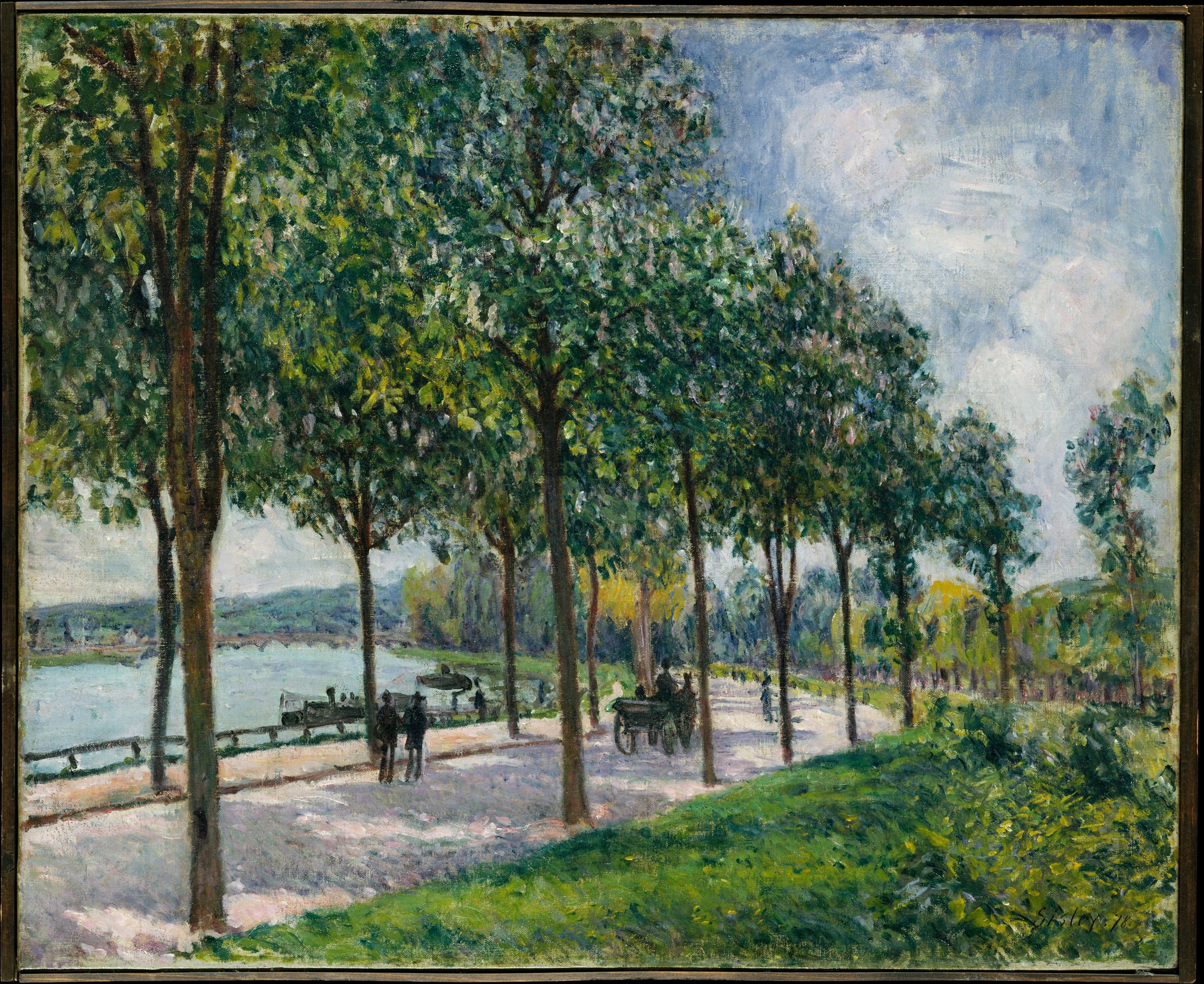
Alfred Sisley, Allée of Chestnut Trees (1878). Oil painting of mature chestnut trees lining a path along the Seine at Sèvres. — Alfred Sisley, *Allée of Chestnut Trees* (1878). The trees in this painting are roughly 80–120 years old. A South Jersey grower planting chestnuts today will not see them this size. Year 5: first nuts. Year 15: mature yield. Year 50+: shape like Sisley saw.
*Oil on canvas, Metropolitan Museum of Art, Robert Lehman Collection — public domain (CC0).*

A new chestnut orchard goes from nothing to full yield —

but most of that climb happens in the first 15 years.

What kind of function shoots up early, then nearly flattens?

And what raises the ceiling itself?

Lesson 17 — IM standards: HSF-IF.C.7.e, HSF-LE.A.4. Two math objectives stay: (1) create graphs of logarithmic functions and use them to answer questions; (2) describe characteristics of logarithmic functions. The redesign topic — chestnut + soil carbon agroforestry — was Mr. Bennett's actual professional domain (former GM, Keystone Tree Crops Cooperative). Use it as the lens, not a swap. Math shape is identical to the IM bacterial-doubling lesson.

Trauma-aware: diffuse / future-tense topic. No student-consent flag needed. If a student says "this is just farming, why is it in algebra?" — affirm: that is the lesson. The math shape of yield-saturation and soil-carbon-saturation is logarithmic. Same math, real ceiling, real money, real intervention levers.

Prep Checklist

☐ Read the Data + Intervention Packet (above) before class.
☐ Graphing technology (Desmos / TI) for Activity 2.
☐ Optional: pull up ktcc.coop in a tab — students may not know what an aggregator co-op is.

Big Question

Why does a logarithmic graph shoot up fast and then nearly flatten out — and what real-world phenomenon looks exactly like that shape?

Today: chestnut yield per acre, and the soil carbon stock under it. Two real things. Same math shape.

Display for ~30 seconds while students settle. Do not solicit answers — this is framing. SWBAT moves to the lesson synthesis (end-of-lesson confirmation), not here.

Warm-Up 5 min

Do Now — Which Three Go Together?

Find as many sets of three as you can. Be ready to explain why.

A $f(x) = 4 \cdot 2^{x}$

B $g(x) = 4 \cdot 10^{x}$

C $h(x) = 2^{x}$

D $k(x) = 4 \cdot \log_{2} x$

Try Saying Functions ___, ___, and ___ go together because ___.

5 min total (slides 3–4). Quiet think 1 min, then group share. There is no single answer. Listen for terminology: increasing, exponential, base, logarithmic. Possible groupings:

A, B, C — the three exponentials (variable in the exponent). D is the odd one out.
A, B, D — coefficient is 4 in front. C is the odd one out.
A, C, D — base is 2. B is the odd one out (base 10).
B, C, D — all increasing functions of x. (A is too.)

Conclude by naming D a logarithmic function — today's topic.

Warm-Up · Synthesis included

Naming the New Shape

Surface a few groupings, then name function D.

“Why is D different from A, B, and C?” A, B, C are exponential — the variable x is the exponent. D is logarithmic — the variable x is inside the log, and the output is the exponent.

“What does $\log_{2} x$ mean in plain language?” "The exponent that 2 must be raised to in order to get x." So $\log_{2} 8 = 3$ (because $2^{3} = 8$), and $\log_{2} 1 = 0$, and $\log_{2} 1024 = 10$.

“If A and D both contain a 4 and a 2, are they the same function?” No. A doubles its output every time x increases by 1. D adds 4 to its output every time x is multiplied by 2. They are inverses in shape: A's growth is D's input scale.

click to advance discussion ▶

Drive the contrast: exponential and logarithmic are opposite kinds of functions. Today we will see a logarithmic function appear from a real-world setup that wants to invert an exponential — namely, "given a population (output), how long did it take to get here (input)?" That setup matches both bacteria and tree yield.

MASL · New Vocabulary

Logarithmic function

Math

$f(x) = \log_{b} x$

We Say

"f of x equals log base b of x"

Meaning

A logarithmic function has the form f(x) = log base b of x, where b is a positive constant. The output is the exponent b must be raised to in order to get x.

Today: base 2 and base 10

Math

$t = \log_{2} p$

We Say

"t equals log base 2 of p"

Meaning

If p doubles every unit of time, then t = log₂p tells you how many doublings have happened.

Math

$d = \log_{10} p$

We Say

"d equals log base 10 of p"

Meaning

If p grows tenfold every unit, then d = log₁₀p tells you how many tenfoldings have happened.

MASL slide first, then How To and work-time. Read each row aloud. Press the spoken phrase: "log base b" — students often drop the word "base." Connection back to Lesson 16: students saw $\log_{2}$ and $\log_{10}$ as operations on numbers; today they appear as functions of x.

Activity 1 · Launch 3 min

How Long Until a Chestnut Orchard Yields?

Mr. Bennett's chestnut orchard starts producing nuts in year 5. After year 5, in this model, the yield doubles every year until it reaches the mature ceiling. Start small: 1 thousand pounds per acre at year 5. Yield P in thousands of pounds per acre.

Setting up the function Let $t$ be the number of years after the orchard hits 1 thousand lbs/acre.
If yield doubles every year: $P = 2^{\,t}$ (thousands of lbs per acre).
Inverted: $\;t = \log_{2} P\;$ — “how many doublings is it?”

Critique & Clarify: A student wrote: "I rewrote the equation as $P = 2^{t}$ because I am trying to find the years for the different values of P." What part is unclear, incorrect, or incomplete?

Launch (~3 min). Read the chestnut setup aloud. The doubling-each-year is a simplifying model — real chestnut yield does not literally double, but it grows fast in the bear-up phase before mature ceiling. Tell students this; do not let them think the model is reality. The IM activity uses bacteria; we use chestnut yield because the math is identical and the orchard is real.

Use Critique, Correct, Clarify on the disc-prompt. The student response is backwards: $P = 2^{t}$ gives P from t, not t from P. The correct rewriting is $t = \log_{2} P$. Students revise with a partner (~2 min) before Activity 1 work-time.

Reference · How To Activity 1 · Work Time 15 min

Reference · How To — Read $t = \log_{2} P$

Step	What to do	Example
1	Read the equation: t = log base 2 of P. Output is years; input is yield (thousands of lbs).	At P = 1 thousand lbs: $t = \log_{2} 1 = 0$ years (the start).
2	Each time P doubles, t increases by 1.	$\log_{2} 2 = 1$, $\log_{2} 4 = 2$, $\log_{2} 8 = 3$, $\log_{2} 16 = 4$.
3	For values of P between powers of 2, the output lies between integers.	$\log_{2} 50$: since $2^{5} = 32$ and $2^{6} = 64$, the answer is between 5 and 6 — closer to 6.
★	Use a calculator: `log(50)/log(2)` = $\log_{2} 50$.	$\log_{2} 50 \approx 5.64$ years.

Activity 1 · Work Time

Problems

Explain why $t = \log_{2} P$ gives the years to reach P thousand lbs/acre — starting from 1 thousand at $t=0$.

Complete the table:

P (thousand lbs/acre)	1	2	4	8	16	32
t (years)	?	?	?	?	?	?

Plot these pairs on a coordinate plane (P on horizontal axis, t on vertical axis). Connect with a smooth curve. Make two observations about the graph's shape.
Use the graph to estimate t when P = 10, 24, and 50 thousand lbs/acre.

15 min · Activity 1 Work Time. Leave on screen during work time.

Problem 1: If $P = 2^{t}$ (yield doubles each year), then to find t from P, take $\log_{2}$ of both sides: $t = \log_{2} P$.
Problem 2 answers: 0, 1, 2, 3, 4, 5.
Problem 3: Curve goes through (1, 0), (2, 1), (4, 2), (8, 3), (16, 4), (32, 5). Two observations: (a) starts at P=1 with t=0; (b) climbs fast in early years, then flattens — large jumps in P add only one more year.
Problem 4: $\log_{2} 10 \approx 3.32$; $\log_{2} 24 \approx 4.58$; $\log_{2} 50 \approx 5.64$ years.

Watch for: students who flip axes (treat t as input). Press: which is input, which is output?

Real-world note Real chestnut yield does not double literally every year. The doubling model is a clean approximation for the bear-up phase. Activity 2 swaps to base-10 and a different scale, then we compare the two graphs.

Amplify · 4 inputs

Order per problem: Text → Math Response (named answer1, answer2 [single check on a representative cell], answer4a, answer4b, answer4c) → Note. Problem 3 = paper graph.

Format examples: Example: 4 · Example: 3.32 · Example: 4.58 · Example: 5.64

Problem 1: Why does t = log₂ P give years? [Text Response]

content:
  when answer1.submitted and not isBlank(answer1.content)
    "Thank you — share your reasoning during synthesis."
  when answer1.submitted and isBlank(answer1.content)
    "Please write a short explanation before submitting."
  otherwise ""

Problem 2: t when P = 16.

content:
  when answer2.submitted and answer2.numericValue = 4
    "Correct! 16 = 2⁴, so log₂ 16 = 4 years."
  when answer2.submitted and answer2.numericValue = 8
    "Almost — 8 is not log₂ 16. log₂ 16 asks: 2 to what power gives 16? 2⁴ = 16."
  when answer2.submitted and not isBlank(answer2.latex)
    "Not quite — log₂ 16 asks: 2 to what power equals 16? Try small whole numbers."
  otherwise ""

Problem 4a: t when P = 10 (calculator allowed).

content:
  when answer4a.submitted and answer4a.numericValue > 3.31 and answer4a.numericValue < 3.33
    "Correct! log₂ 10 ≈ 3.32 years. Between log₂ 8 = 3 and log₂ 16 = 4, closer to 3."
  when answer4a.submitted and answer4a.numericValue > 0.99 and answer4a.numericValue < 1.01
    "Almost — log₁₀ 10 = 1, but the question asks log₂ 10. Use log(10)/log(2) on a calculator."
  when answer4a.submitted and not isBlank(answer4a.latex)
    "Hmm... take another look — log₂ 10 lies between log₂ 8 = 3 and log₂ 16 = 4. Compute log(10)/log(2) on a calculator."
  otherwise ""

Problem 4b: t when P = 24.

content:
  when answer4b.submitted and answer4b.numericValue > 4.57 and answer4b.numericValue < 4.59
    "Correct! log₂ 24 ≈ 4.58 years. Between log₂ 16 = 4 and log₂ 32 = 5."
  when answer4b.submitted and answer4b.numericValue > 11.99 and answer4b.numericValue < 12.01
    "Not quite — 12 is half of 24, not log₂ 24. log₂ 24 asks: 2 to what power gives 24? Closer to 4.58."
  when answer4b.submitted and not isBlank(answer4b.latex)
    "Almost — log₂ 24 lies between 4 (since 2⁴ = 16) and 5 (since 2⁵ = 32). Compute log(24)/log(2)."
  otherwise ""

Problem 4c: t when P = 50.

content:
  when answer4c.submitted and answer4c.numericValue > 5.63 and answer4c.numericValue < 5.65
    "Correct! log₂ 50 ≈ 5.64 years. Between log₂ 32 = 5 and log₂ 64 = 6."
  when answer4c.submitted and answer4c.numericValue > 24.99 and answer4c.numericValue < 25.01
    "Almost — 25 is half of 50, not log₂ 50. The log₂ asks for the exponent on 2 that yields 50."
  when answer4c.submitted and not isBlank(answer4c.latex)
    "You're close — log₂ 50 lies between 5 (2⁵ = 32) and 6 (2⁶ = 64). Try log(50)/log(2)."
  otherwise ""

Activity 1 · Synthesis 5 min

The Shape of $t = \log_{2} P$

Surface what students noticed about this shape, and connect it back to the bacteria-doubling intuition.

“What does the input P mean? What does the output t mean?” Input P: yield in thousands of lbs per acre. Output t: how many years of doubling from the 1 thousand lb baseline. $\log_{2} 50 \approx 5.64$ means: about 5.6 years to grow from 1 thousand to 50 thousand lbs/acre — under this doubling-each-year model.

“How is this graph different from an exponential graph?” An exponential climbs steeply at the right; this log graph climbs steeply at the left. Equal-distance jumps along the curve multiply P by the base — they don't add a fixed amount. Going from P=4 to P=8 is one more year. Going from P=16 to P=32 is also one more year — even though the second jump covers 16 thousand more lbs compared to the first jump's 4 thousand.

“Real chestnut yield doubles each year for how long, in your gut?” Not very long. Real orchards bear up rapidly years 5–12, then bend toward a mature ceiling of ~2,000 lbs/acre. The doubling model breaks before the ceiling. That's exactly what a real log-shaped yield curve looks like — fast in, then flat. Activity 2 looks at a slower base.

click to advance discussion ▶

Try Saying The output t means ___ because ___.

Try Saying The graph climbs steeply at first because ___, and flattens because ___.

The IM lesson uses bacteria; we use chestnut yield. Same math, more relevant context. Do not hide the gap between the model and reality — students should see that the model is approximate. The next activity introduces a different base and pushes them to interpret what changing the base means.

Activity 2 · Launch 3 min

Soil Carbon Under the Orchard

Below the chestnut canopy, the soil itself is changing. Under continuous regen practice (no-till, cover crops, manure, tree litter), soil organic carbon (SOC) climbs slowly toward a saturation ceiling. For our model, suppose SOC stock multiplies by 10 over each unit of compounded effort, starting at 1 unit.

Setting up the function Let p = SOC stock relative to baseline (so p = 1 is the start).
Define a function f: $\;f(p) = \log_{10} p\;$ — “how many tenfoldings of SOC?”

Notice: this is the same kind of function as Activity 1, but the base is different (10 instead of 2). What do you predict will be different about its graph?

Connect to Activity 1: same function form, different base. Do not resolve the prediction question yet — students will graph and compare in the work time.

Real-world note for students who push back: SOC does not literally tenfold. The model is a stand-in for a ladder of compounded management effort (no-till × cover crop × manure × tree litter × rotation × …). Each rung roughly tenfolds the durable carbon pool — until you hit the saturation ceiling determined by your soil's mineralogy (Cardinael et al. 2017; Lal 2018).

Activity 2 · Work Time 7 min

$f(p) = \log_{10} p$, where p = SOC stock relative to baseline.

Problems · use graphing tech (Desmos / TI)

Describe how SOC stock changes per unit increase of $f(p)$. (What does adding 1 to f do to p?)
Graph $f(p) = \log_{10} p$. Make two observations about the graph.
Estimate $f(50)$ and $f(20{,}000)$. What does each value mean about SOC?
Estimate the SOC stock p after 5 "tenfoldings of effort" (i.e., when $f = 5$).
Will the graph ever have a point where p is negative? Why or why not?

Try Writing Adding 1 to $f(p)$ means ___ to p, because ___.

7 min · Activity 2 Work Time. Adjust graphing window — students may need to zoom out for problem 4.

Problem 1: Adding 1 to f means multiplying p by 10. (Each tenfolding of p raises f by 1.)
Problem 2: Curve through (1,0), (10,1), (100,2), (1000,3). Steep early, then visibly flat.
Problem 3: $f(50) \approx 1.7$ — about 1.7 tenfoldings have happened. $f(20{,}000) \approx 4.3$ — about 4.3 tenfoldings.
Problem 4: If $f = 5$, then $p = 10^{5} = 100{,}000$. Note: the input has to grow 100,000-fold for f to reach 5. This is the saturation phenomenon.
Problem 5: No. $\log_{10}$ of a negative number is undefined. The domain of f is $p > 0$.

Watch for Students who try to read f(20,000) directly off the graph will need to expand the domain. Press the takeaway: each additional tenfolding of p only adds 1 to f. That's the saturation shape.

Amplify · 4 inputs

Order per problem: Text → Math Response (named answer3a, answer3b, answer4) → Note. Problems 1, 2, 5 = paper / discussion / Text Response.

Format examples: Example: 1.7 · Example: 4.3 · Example: 100000

Problem 3a: f(50) ≈ ?

content:
  when answer3a.submitted and answer3a.numericValue > 1.69 and answer3a.numericValue < 1.71
    "Correct! log₁₀ 50 ≈ 1.70. About 1.7 tenfoldings of SOC have happened."
  when answer3a.submitted and answer3a.numericValue > 1.39 and answer3a.numericValue < 1.41
    "You're close — log₁₀ 25 ≈ 1.40, but the question asks log₁₀ 50. Try log(50) on a calculator."
  when answer3a.submitted and answer3a.numericValue > 24.99 and answer3a.numericValue < 25.01
    "Hmm — 25 is half of 50, but log₁₀ 50 asks: 10 to what power gives 50? It is between 1 (10¹=10) and 2 (10²=100)."
  when answer3a.submitted and not isBlank(answer3a.latex)
    "Almost — log₁₀ 50 lies between 1 (10¹=10) and 2 (10²=100). Use a calculator: log(50)."
  otherwise ""

Problem 3b: f(20,000) ≈ ?

content:
  when answer3b.submitted and answer3b.numericValue > 4.29 and answer3b.numericValue < 4.31
    "Correct! log₁₀ 20,000 ≈ 4.30 — about 4.3 tenfoldings."
  when answer3b.submitted and answer3b.numericValue > 3.99 and answer3b.numericValue < 4.01
    "You're close — log₁₀ 10,000 = 4. log₁₀ 20,000 is a little more (about 4.3) because 20,000 = 2 · 10,000."
  when answer3b.submitted and not isBlank(answer3b.latex)
    "Almost — 20,000 is between 10⁴ = 10,000 and 10⁵ = 100,000. So log₁₀ 20,000 is between 4 and 5."
  otherwise ""

Problem 4: SOC stock p when f = 5.

content:
  when answer4.submitted and answer4.numericValue > 99999 and answer4.numericValue < 100001
    "Correct! If f = 5, then p = 10⁵ = 100,000. Five tenfoldings of effort to get there. Notice: the input had to climb 100,000-fold to make f reach 5 — that's the saturation shape."
  when answer4.submitted and answer4.numericValue > 9999 and answer4.numericValue < 10001
    "Almost — 10,000 = 10⁴, so f = 4 there. For f = 5, p must be 10⁵."
  when answer4.submitted and answer4.numericValue > 49 and answer4.numericValue < 51
    "Hmm... 50 is the input, not 5. The question asks: when f = 5, what is p? p = 10⁵."
  when answer4.submitted and not isBlank(answer4.latex)
    "Not quite — if log₁₀ p = 5, then p = 10⁵. What is 10⁵?"
  otherwise ""

Problem 5: Will p ever be negative? [Text Response]

content:
  when answer5.submitted and not isBlank(answer5.content)
    "Thank you — share your reasoning during synthesis."
  when answer5.submitted and isBlank(answer5.content)
    "Please write a short explanation before submitting."
  otherwise ""

Activity 2 · Synthesis 5 min

Two Bases, Two Curves — Same Shape

Both curves shoot up fast at the start, then bend hard toward flat. Same shape. Different base changes how fast you reach each step.

“Which curve climbs faster, and why?” $\log_{2}$ (blue, chestnut) climbs faster early. Each doubling of p raises t by 1. $\log_{10}$ (green, SOC) is slower — p has to tenfold to raise f by 1. Both are increasing functions; both flatten as p grows large; $\log_{10}$ just flattens harder.

“What's the same about the two graphs?” Both pass through (1, 0) (any base raised to the 0 is 1). Both are defined only for p > 0 (no negative inputs). Both increase forever — but slowly. Each one's input has to multiply by the base to advance the output by 1.

“What real story does each curve tell?” Blue ($\log_{2}$, chestnut yield): a young orchard's bear-up phase. Yield doubles annually for a window — roughly years 5 to 12 — then bends. Real ceiling: ~2,000 lbs/acre. The flatness is biological maturity.

Green ($\log_{10}$, soil organic carbon): the slow stable carbon pool under continuous regen practice. Each "tenfold" of compounded effort climbs the curve by 1. Eventually you hit soil-mineral saturation — there is only so much carbon a given soil can hold. The flatness is a physical ceiling.

click to advance discussion ▶

Try Saying Base ___ climbs faster than base ___ because ___.

The IM lesson highlights two things: (a) input must multiply by b to advance output by 1; (b) both graphs pass through (1, 0). Make sure both land. The "real story" reveal is the agency setup — students need to understand that the ceiling is real before we ask them to push on it. Next slide: agency move.

Agency Move 7 min

What raises the ceiling?

The flatness in both curves is a ceiling: chestnut biology, soil-carbon mineralogy. A 16-year-old grower in South Jersey cannot change the shape of the log curve — but real interventions shift the ceiling itself (raising mature yield, raising soil's carbon-holding capacity, or paying for the slow climb).

EQIP Practice 612 — Tree/Shrub Establishment

Cost-share for the planting itself. Covers 45–75% of typical NJ establishment cost. USDA NRCS Mid-Atlantic, FY 2025.

EQIP Practice 311 — Alley Cropping

Pays per-acre to integrate trees with row crops on the same parcel. $20.80–$88.50/acre (PA & DC FY23). NRCS state payment schedules.

Climate-Smart Commodities (2022–2027)

$3.1 B across 141 partnerships; agroforestry projects layer on top of EQIP. Per-acre stewardship payments, multi-year. USDA, Sept 2022 + Oct 2024.

Conservation Reserve Program (CRP)

10–15-year contracts for taking land out of row crops; de-risks the planting-to-yield gap. ~$50–$300/acre/yr depending on county. USDA FSA.

Carbon credit revenue (regen-ag protocols)

Voluntary markets pay for verified sequestration. ~$55–$110/acre/yr at $15–$30 per tCO₂e. Voluntary carbon market, 2024–2025.

Cooperative aggregator (KTCC)

Member-owned PA processor for chestnut flour, hickory + hazel oil. Raises farm-gate $/lb by aggregating supply. Keystone Tree Crops Cooperative, ktcc.coop.

Pick one. Which lever moves the ceiling fastest? Popcorn discussion — 60 seconds, then we ask the rate question.

Try Saying I would push for ___ because it raises ___ by ___, which shifts the curve so that ___.

7 min — agency move. Read the framing aloud. Give 60 seconds quiet, then 60 seconds popcorn share. Sequence the discussion so multiple cards get named — not the same one repeated.

The math link: the log curve has a flat tail because each step requires multiplying the input by the base. Interventions do not change the base — but they can:

raise the asymptote (CRP buys time so the slow stable carbon pool can fill);
raise mature yield (KTCC raises $/lb so 2,000 lbs/acre × higher price = more revenue per ceiling unit);
pay for the climb itself (EQIP 612 / 311 + Climate-Smart) so the grower survives the 10-year zero-yield window.

Press the rate question next slide. Don't moralize. Don't despair-theater. The numbers are real; the levers are real.

Trauma-aware: students may have farming families, foreclosure history, or none of the above. Don't ask for personal stories. The intervention cards are policy levers, not personal asks.

Lesson Synthesis 3 min

The Rate Question to Leave With

A new chestnut planting reaches mature yield (~2,000 lbs/acre) at year 15 — only if the grower survives years 5–14 with low yield. EQIP + CRP + carbon revenue close the gap.

“Look at the two graphs from Activity 2. Which one's flat tail is more dangerous to the grower — and why?” Both flatten, but for different reasons. Yield curve ($\log_{2}$) flattens because the tree biologically caps out — the grower can't push past mature yield without grafting better cultivars. SOC curve ($\log_{10}$) flattens because soil saturates — the grower can't sequester past the mineralogy ceiling. Both are real ceilings. The danger is mistaking the flat tail for the early steep climb — interventions need to fund the climb, not chase the tail.

“If you graph $t = \log_{2} P$ and $t = \log_{10} P$ on the same axes, which is on top for P > 1?” $\log_{2}$ is on top. For any P > 1, $\log_{2} P$ > $\log_{10} P$, because each doubling (base 2) is a smaller multiplicative step than each tenfolding (base 10). So fewer steps of size 10 fit in the same input range — the base-10 curve grows slower.

“Sentence frame for closing: which intervention, and what number does it raise the ceiling by?” Sample student responses (real numbers from the packet):

"EQIP 612 covers 45–75% of planting cost — that lets a small grower in NJ start at all."
"CRP at $200/acre/yr × 10 years = $2,000/acre to bridge the no-yield gap."
"KTCC raises farm-gate by aggregating supply — same yield × higher $/lb = higher revenue ceiling."
"Carbon credits at $80/acre/yr layered on top means the soil carbon side also pays."

click to advance discussion ▶

Try Saying For a 10-acre orchard in South Jersey, the lever I would push first is ___ because it raises ___ by ___ before mature yield arrives.

I Can… (SWBAT)

Create a graph of a logarithmic function and use it to answer questions about the situation it models.

Describe characteristics of logarithmic functions — domain, behavior at x = 1, slow growth at large x, and how the base changes the rate.

Lesson Synthesis — confirmation, not preview. Do not resolve the third question for students; it's the bring-home rate question. Teacher can collect named-intervention sentences as exit ticket.

The math objectives close here: students can read a log graph, state the base's effect on the rate, and translate "input multiplies by b" into "output adds 1." Tomorrow's lesson (Lesson 18, IM section D) extends to logarithmic equations algebraically.

Reference · How To Cool-Down 5 min

Reference · How To — Identify which graph is which base

Step	What to do	Example
1	Pick a known point on each curve, ideally at x = 100 or another power of the suspected base.	Read off the output at x = 100.
2	If output ≈ 2 at x = 100, the curve is $\log_{10}$ (because $10^{2} = 100$).	$\log_{10} 100 = 2$ ✓
3	If output is between 6 and 7 at x = 100, the curve is $\log_{2}$ (because 100 lies between $2^{6}$ = 64 and $2^{7}$ = 128).	$\log_{2} 100 \approx 6.64$ ✓
★	Both curves pass through (1, 0). Use that as your anchor when an axis label is partly cut off.	Any base b: $\log_{b} 1 = 0$.

Cool-Down · 5 min

Two curves are graphed below. They represent $g(x) = \log_{2} x$ and $h(x) = \log_{10} x$.

Use the labeled points to determine which curve is $g(x)$ and which is $h(x)$. Explain how you know.
Use the graph to estimate $\log_{10} 100$ and $\log_{2} 100$.

Cool-Down · 5 min. Students apply the lesson's central skill: read a log curve and identify the base from a known point. Leave the How To slide on screen during the cool-down.

Problem 1: Curve A goes through (100, 6.64) — that is $\log_{2} 100$ (since 2⁶=64, 2⁷=128). So Curve A is $g(x) = \log_{2} x$. Curve B goes through (100, 2) — that is $\log_{10} 100$ (since 10²=100). Curve B is $h(x) = \log_{10} x$.

Problem 2: $\log_{10} 100 = 2$ (exact). $\log_{2} 100 \approx 6.64$.

Amplify · Cool-Down (3 inputs)

Order: Text → Math Response (named answer1, answer2a, answer2b) → Note. Problem 1 explanation → Text Response (answer1exp).

Format examples: Example: A is g(x), B is h(x) · Example: 2 · Example: 6.64

Problem 1 explanation: How can you tell A from B? [Text Response]

content:
  when answer1exp.submitted and not isBlank(answer1exp.content)
    "Thank you. Key idea: Curve A passes through (100, 6.64), and 2⁶ = 64, 2⁷ = 128, so log₂ 100 ≈ 6.64. Curve B passes through (100, 2), and 10² = 100, so log₁₀ 100 = 2."
  when answer1exp.submitted and isBlank(answer1exp.content)
    "Please write a short explanation before submitting."
  otherwise ""

Problem 2a: Estimate log₁₀ 100.

content:
  when answer2a.submitted and answer2a.numericValue = 2
    "Correct! log₁₀ 100 = 2 (exactly), because 10² = 100."
  when answer2a.submitted and answer2a.numericValue > 1.99 and answer2a.numericValue < 2.01
    "Correct! log₁₀ 100 ≈ 2."
  when answer2a.submitted and answer2a.numericValue > 6.5 and answer2a.numericValue < 6.7
    "Almost — that is log₂ 100, not log₁₀ 100. Check the base. 10 to what power gives 100?"
  when answer2a.submitted and answer2a.numericValue = 100
    "Hmm — 100 is the input, not the log. log₁₀ 100 asks: 10 to what power equals 100? Try a small whole number."
  when answer2a.submitted and not isBlank(answer2a.latex)
    "Almost — log₁₀ 100 asks: 10 to what power gives 100?"
  otherwise ""

Problem 2b: Estimate log₂ 100.

content:
  when answer2b.submitted and answer2b.numericValue > 6.63 and answer2b.numericValue < 6.65
    "Correct! log₂ 100 ≈ 6.64 — between log₂ 64 = 6 and log₂ 128 = 7."
  when answer2b.submitted and answer2b.numericValue > 6.59 and answer2b.numericValue < 6.69
    "Correct (close enough). log₂ 100 ≈ 6.64."
  when answer2b.submitted and answer2b.numericValue = 2
    "Almost — that is log₁₀ 100, not log₂ 100. Different base. log₂ 100 lies between 6 (2⁶=64) and 7 (2⁷=128)."
  when answer2b.submitted and answer2b.numericValue = 50
    "Hmm — 50 is half of 100, not log₂ 100. Try log(100)/log(2) on a calculator."
  when answer2b.submitted and not isBlank(answer2b.latex)
    "Almost — log₂ 100 lies between 6 (2⁶ = 64) and 7 (2⁷ = 128). Use log(100)/log(2)."
  otherwise ""

Lesson Summary

A logarithmic function inverts the question.

Earlier we wrote exponential functions where the input is the exponent and the output grows fast. Today we wrote logarithmic functions — $f(x) = \log_{b} x$ — where the output is the exponent and the input is what we want to undo. "b raised to what power gives x?"

Chestnut yield (base 2)

$t = \log_{2} P$ — each year that passes, yield doubles. Steep early; flat by year ~12.

Soil carbon (base 10)

$f = \log_{10} p$ — input must tenfold to advance output by 1. Saturation is real.

The Wrench

Interventions don't change the base. They raise the ceiling or fund the climb.

Lesson Summary A logarithmic function $f(x) = \log_{b} x$ inverts an exponential. It is defined for x > 0, passes through (1, 0), grows forever, and grows slower the larger x gets. The base determines how slow.

Lesson Summary — read aloud or have a student read. Tomorrow (IM Lesson 18) extends to algebraic manipulation of log equations. Carry forward the takeaway: the math reveals trajectories; the agency move asks what shifts them.

Topic — Chestnut yield + soil carbon saturation in agroforestry

Key data points (citations below)

Interventions with measured effect sizes

Sources

Logarithmic Functions

Why does a logarithmic graph shoot up fast and then nearly flatten out — and what real-world phenomenon looks exactly like that shape?

Do Now — Which Three Go Together?

Naming the New Shape

Logarithmic function

How Long Until a Chestnut Orchard Yields?

The Shape of \(t = \log_{2} P\)

Soil Carbon Under the Orchard

Two Bases, Two Curves — Same Shape

What raises the ceiling?

EQIP Practice 612 — Tree/Shrub Establishment

EQIP Practice 311 — Alley Cropping

Climate-Smart Commodities (2022–2027)

Conservation Reserve Program (CRP)

Carbon credit revenue (regen-ag protocols)

Cooperative aggregator (KTCC)

The Rate Question to Leave With

A logarithmic function inverts the question.

Step	What to do	Example
1	Read the equation: t = log base 2 of P. Output is years; input is yield (thousands of lbs).	At P = 1 thousand lbs: \(t = \log_{2} 1 = 0\) years (the start).
2	Each time P doubles, t increases by 1.	\(\log_{2} 2 = 1\), \(\log_{2} 4 = 2\), \(\log_{2} 8 = 3\), \(\log_{2} 16 = 4\).
3	For values of P between powers of 2, the output lies between integers.	\(\log_{2} 50\): since \(2^{5} = 32\) and \(2^{6} = 64\), the answer is between 5 and 6 — closer to 6.
★	Use a calculator: `log(50)/log(2)` = \(\log_{2} 50\).	\(\log_{2} 50 \approx 5.64\) years.

Step	What to do	Example
1	Pick a known point on each curve, ideally at x = 100 or another power of the suspected base.	Read off the output at x = 100.
2	If output ≈ 2 at x = 100, the curve is \(\log_{10}\) (because \(10^{2} = 100\)).	\(\log_{10} 100 = 2\) ✓
3	If output is between 6 and 7 at x = 100, the curve is \(\log_{2}\) (because 100 lies between \(2^{6}\) = 64 and \(2^{7}\) = 128).	\(\log_{2} 100 \approx 6.64\) ✓
★	Both curves pass through (1, 0). Use that as your anchor when an axis label is partly cut off.	Any base b: \(\log_{b} 1 = 0\).